T-SNE
seqlearner.MultiTaskLearner.visualize(method="TSNE", family=None, proportion=1.5)
t-Distributed Stochastic Neighbor Embedding (t-SNE) is a (prize-winning) technique for dimensionality reduction that is particularly well suited for the visualization of high-dimensional datasets. The technique can be implemented via Barnes-Hut approximations, allowing it to be applied on large real-world datasets.
You can find more information about this technique and its variants are introduced in the following papers: - L.J.P. van der Maaten. Accelerating t-SNE using Tree-Based Algorithms. Journal of Machine Learning Research 15(Oct):3221-3245, 2014. - L.J.P. van der Maaten and G.E. Hinton. Visualizing Non-Metric Similarities in Multiple Maps. Machine Learning 87(1):33-55, 2012. - L.J.P. van der Maaten. Learning a Parametric Embedding by Preserving Local Structure. In Proceedings of the Twelfth International Conference on Artificial Intelligence & Statistics (AI-STATS), JMLR W&CP 5:384-391, 2009. - L.J.P. van der Maaten and G.E. Hinton. Visualizing High-Dimensional Data Using t-SNE. Journal of Machine Learning Research 9(Nov):2579-2605, 2008.
We have used the sklearn wrapper function which implements T-SNE and applied it on the embedding results.
The visualize method has the following arguments:
Arguments
- method: String, Possible values are
TSNEandUMAP - family: String, Name of protein family to be visualized
- proportion: Positive float, population proportion of number of other classes by number of
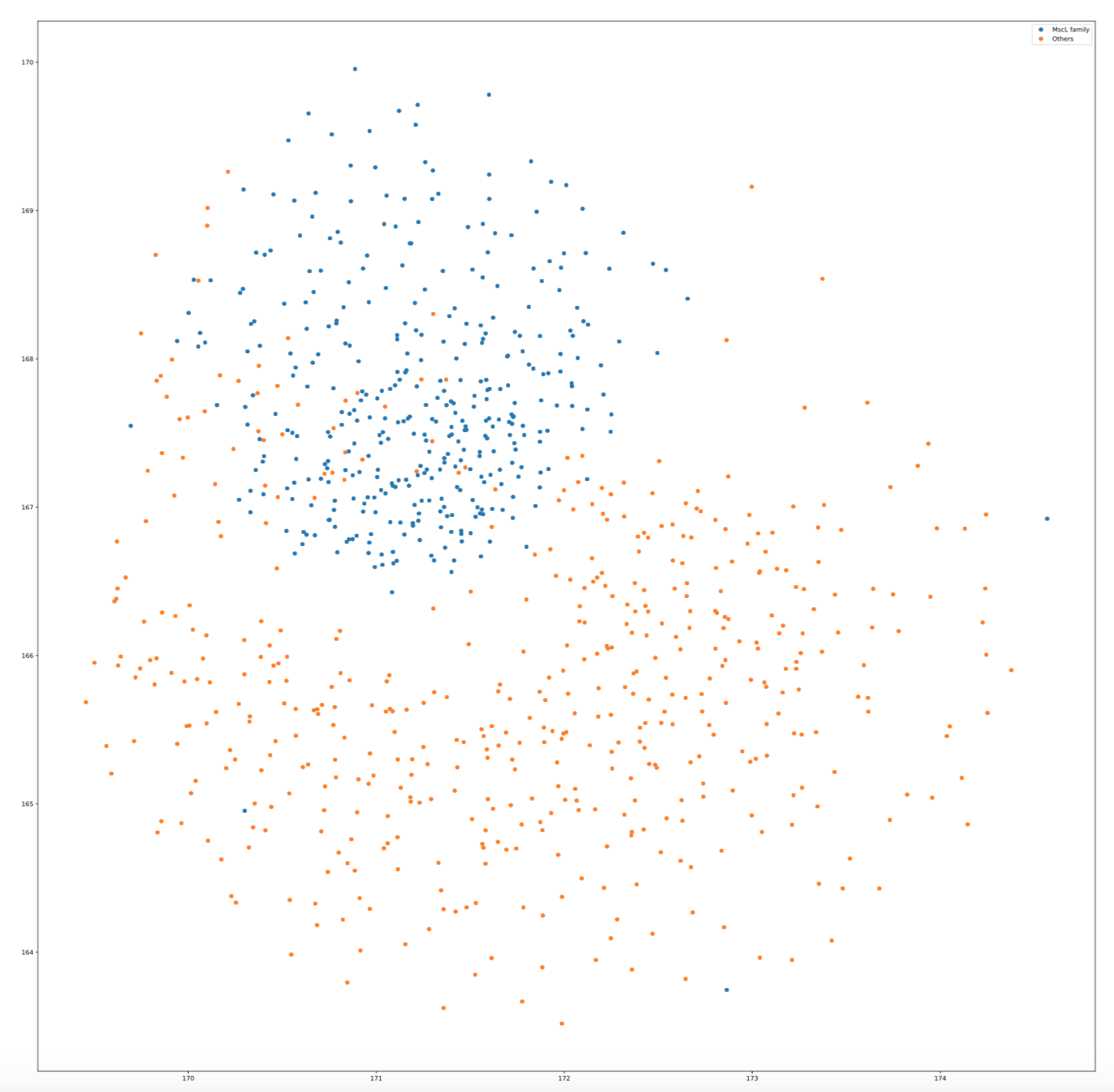
Apply T-SNE visualization on MscL protein family
from seqlearner import MultiTaskLearner as mtl
import pandas as pd
from seqlearner import Freq2Vec
sequences = pd.read_csv("./protein_sequences.csv", header=None)
freq2vec = Freq2Vec(sequences, word_length=3, window_size=5, emb_dim=25, loss="mean_squared_error", epochs=250)
freq2vec.freq2vec_maker()
freq2vec_embedding = mtl.embed(word_length=3, embedding="freq2vec", func="sum", emb_dim=25, gamma=0.1, epochs=100)
mtl.visualize(method="TSNE", family="MscL_family", proportion=2.0)
The visualization plot is in the following: